·35 min read· architecture· pre-training· scaling laws
I Tried Every LLM Architecture Change since 2020
The best architecture change since GPT-3 is fine-grained MoE, linear attention and hyper-connections work.
Architecture research is one of the highest aura jobs you can have right now. Open a tech report and architecture gets a huge chunk of it. There's also this mystery around it, like all this stuff was invented by some gigabrains who look at raw tensor printouts, see the norm blowups, and come up with manifold-constrained hyperconnectors or whatever.
It's also a pain to compare architectures properly, for three reasons:
- There is no clear definition of what "an architecture A is better than architecture B" is. Better how? Better loss per parameter? Cheaper to serve? Cheaper to train? A combination of these factors? Something else?
- The results that do exist are very setup dependent. All the signals flip depending on how strong you value long context, what data you use, what hardware you have, how the inference load looks like, etc.
- As almost all things in LLMs, the results loosely transfer with scale. Whenever you see a new nanoGPT-speedrun record, the first question you ask is "does it scale?".
There are also opinions that architecture probably isn't that important. That the data and proper pre-training (and especially post-training) setup tuning is where the big wins are. All the rumors that frontier labs are training the most boring transformers ever, that "pre-training is dead", and all this "old data, modern arch vs modern data, old arch" discourse.
I wanted to put the architecture decisions that open labs and researchers made over the last six years into the same setup and see which ones held up.
So I ran more than 1,000 experiments, trying the changes on their own and then stacking the winners to see how much of the improvement survived.
I'd been thinking about this "mega-ablation" for over a year. Coding agents finally made it doable in a reasonable amount of time.
I trained all these weird models with bux, the framework I built for architecture experiments. You can define an architecture, train it, export it to vLLM, and measure both quality and inference speed.
#Setup
I trained on a mix of code files and whole Python repositories from Stack-Edu, plus web text from FineWeb-Edu, using AdamW. Training starts with 2k-token sequences and ends with a 16k context extension. The recipe:
- Shapes. Every model keeps GPT-3's proportions: one layer per 64 of width, and attention heads of 64. We train up to four widths: d_model 512, 768, 1024 and 1280. For the GPT-3 baseline that's 25M to 394M non-embedding parameters.
- Same tokens for everyone. At a given width, every model reads the same tokens: 20 per non-embedding parameter of the GPT-3 baseline at that width. That's 0.5B, 1.7B, 4.0B and 7.9B tokens.
- Training. AdamW with weight decay 0.1, a warmup-stable-decay schedule (5% warmup, 20% decay), z-loss 1e-4, the GPT-NeoX tokenizer. The batch follows DeepSeek's batch-size law: 48 to 288 rows of 2k tokens.
- Long context. The first 90% of steps use rows of 2k tokens: 60% code, 40% web. The last 10% use rows of 16k: 50% whole repositories, 30% code, 20% web. At the switch, every full-attention layer with RoPE gets YaRN (8x).
- Hardware. B300 GPUs. The smallest run takes about 10 minutes on one GPU; the largest takes about 14 hours on four.
Each architecture gets a short learning-rate sweep: 1e-3, 2e-3 and 4e-3 at , plus 8e-3 for changes that claim to help stability. I fit a parabola in log learning rate and reuse its minimum at the wider models.
I measure quality in bits per byte (BPB) on held-out data: 0.5 × code files + 0.3 × whole repositories + 0.2 × web text. Repositories are read in 16k-token windows, so long context counts. Lower is better: -2% means 2% fewer bits per byte.
Changing only the seed moves the objective by about 0.7%. Runs with the same seed see the same data in the same order, so we always compare runs that share a seed. That cuts the noise of a comparison to about 0.3%.
At Mellum, I cared about how good a model we could get within our inference constraints. So I give every architecture the same serving budget. If a change makes serving cheaper, I spend the savings on a bigger model.
The baseline is GPT-3-like: GPT-3 6.7B's shape, d_model 4096, 32 layers and full multi-head attention. It runs in vLLM 0.32 with bux's plugin, FP8 weights, activations and KV cache, on one B300. The workload roughly simulates a coding agent: each session gets a shared 2k-token prefix, 14k tokens of its own context, then 4 turns where the model writes 512 tokens and gets a 2k-token tool result back. Prefix caching is on.
I count how many sessions per hour per GPU it can handle while median time per output token stays under 30 ms. The baseline does 1,924 sessions/h. Each architecture has to match that, and I measure how big a model it can afford.
I train two to four small models per architecture: and for every change, plus and for the promising ones. Then I fit a scaling law to predict their quality at the size that matches the serving budget:
- We measure the target inference size. I export each architecture from bux without weights at 3-4 sizes and time each one in vLLM under the same load. Interpolating between them gives the size at which it serves exactly 1,924 sessions/h per GPU. That size is the architecture's target. The 2021 reference (GPT-3 + RoPE) gets 3.7B active parameters, GQA gets 13.8B, and the 2026 KDA hybrid gets 11.4B active (201B total). I tried an analytic cost model first. It was right on the median but far off wherever kernels matter (sparse attention, MLA), so I use it only to choose which sizes to time.
- The law. We fit to all families at once, where N is the active non-embedding parameters and D the tokens. E, the entropy of the data, is fixed from an earlier ladder on the same data. B and β are shared, since everyone sees the same data. A is always a family's own. α is its own only with 3+ widths; otherwise it borrows its parent's.
- Two numbers per change. "Worth N times its parameters" compares models at the trained sizes. "Change at equal serving cost" reads the law at the target size and 1T tokens. These two often disagree.
Disclaimer: don't treat this as an actual scientific study or trust the results more than the setup allows for. The obvious concerns are:
- The serving cost heavily depends on how optimized the inference stack (in my case, vLLM) is for this particular architecture.
- The scaling ladder is tiny and we extrapolate very far for the target size.
- The data is toy, as well as the quality benchmarks, the training setup is quite far from the production one, e.g., we only extend to 16k.
- I didn't tune all the hyperparameters and didn't sweep all the method options.
- The code was largely written by Claude Opus 5.5, which is a very good model, but take it with a grain of salt.
- I intended it as a fun evening project.
#Results
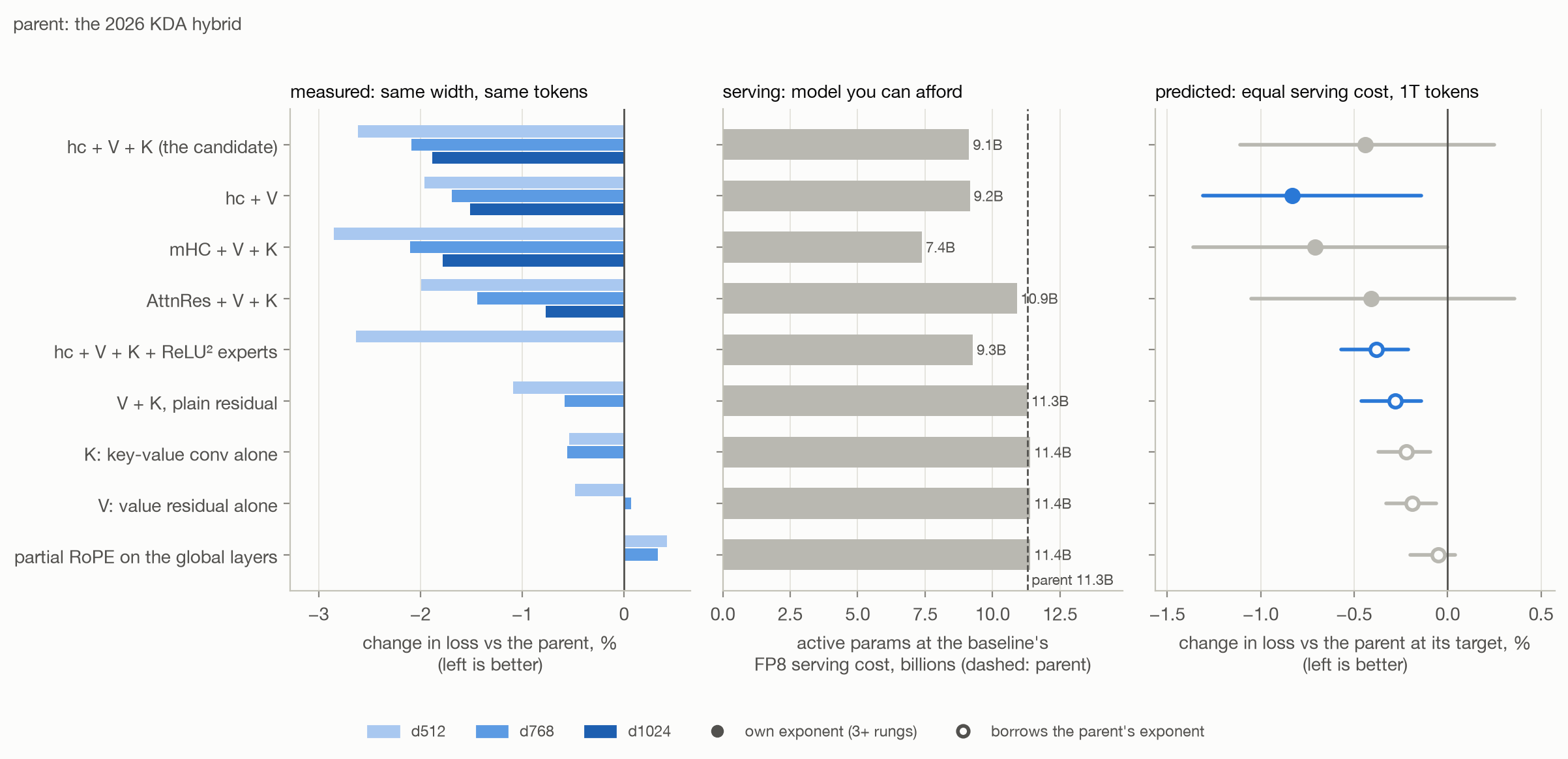
Before getting into individual changes, a quick explanation of the plots. Each has up to three panels:
- Measured: what happened when I trained the model with this change, compared to the model without it, at the same width and token budget. The bars go from to to , light to dark.
- Serving: how many active parameters I can serve for the same cost as the baseline. The dashed line is the model before the change.
- Predicted: what the scaling-law fit thinks the change would do at that serving size, after training on 1T tokens. Blue means the whole predicted range is below zero, red means above, gray means it crosses zero. Hollow dots are the ones where I only trained two widths and had to reuse the original model's scaling exponent. I'd be especially careful with those.
The first panel is what I measured on small models. The third is an extrapolation to much bigger ones, with all the problems I listed above. The loss changes at equal serving cost below come from that third panel.
There are also three models I'll keep referring to:
- The 2021 reference is GPT-3 with RoPE instead of learned positions. Unless I say otherwise, this is the model I apply each individual change to.
- The 2026 hybrid is a small version of a late-2026 architecture: three KDA layers for every global attention layer, fine-grained MoE, QK-norm, gated attention and MTP. This is where I start combining changes.
- The candidate is what I call the hybrid after adding hyper-connections (HC: four copies of the residual stream), a value residual (V) and Inkling's key-value conv (K) on the global layers. I use it for the later stacking rounds, sparse attention and Canon experiments. The final model is this one with its dense FFN moved from the first layer to the last.
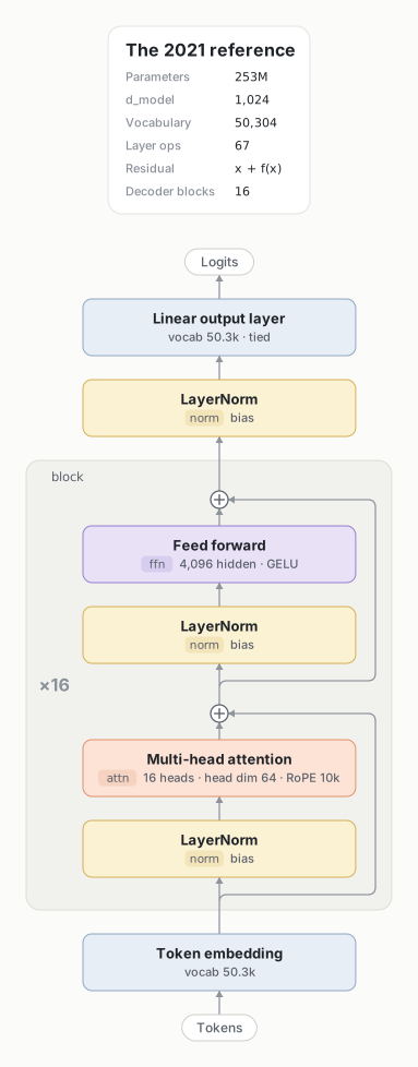
The reference, drawn in bux studio. All four architecture diagrams use and 16 decoder blocks. Tokens flow from bottom to top; ×n repeats a block. Click any figure to open it at full size. Diagram source.
#Individual Changes
#High level overview
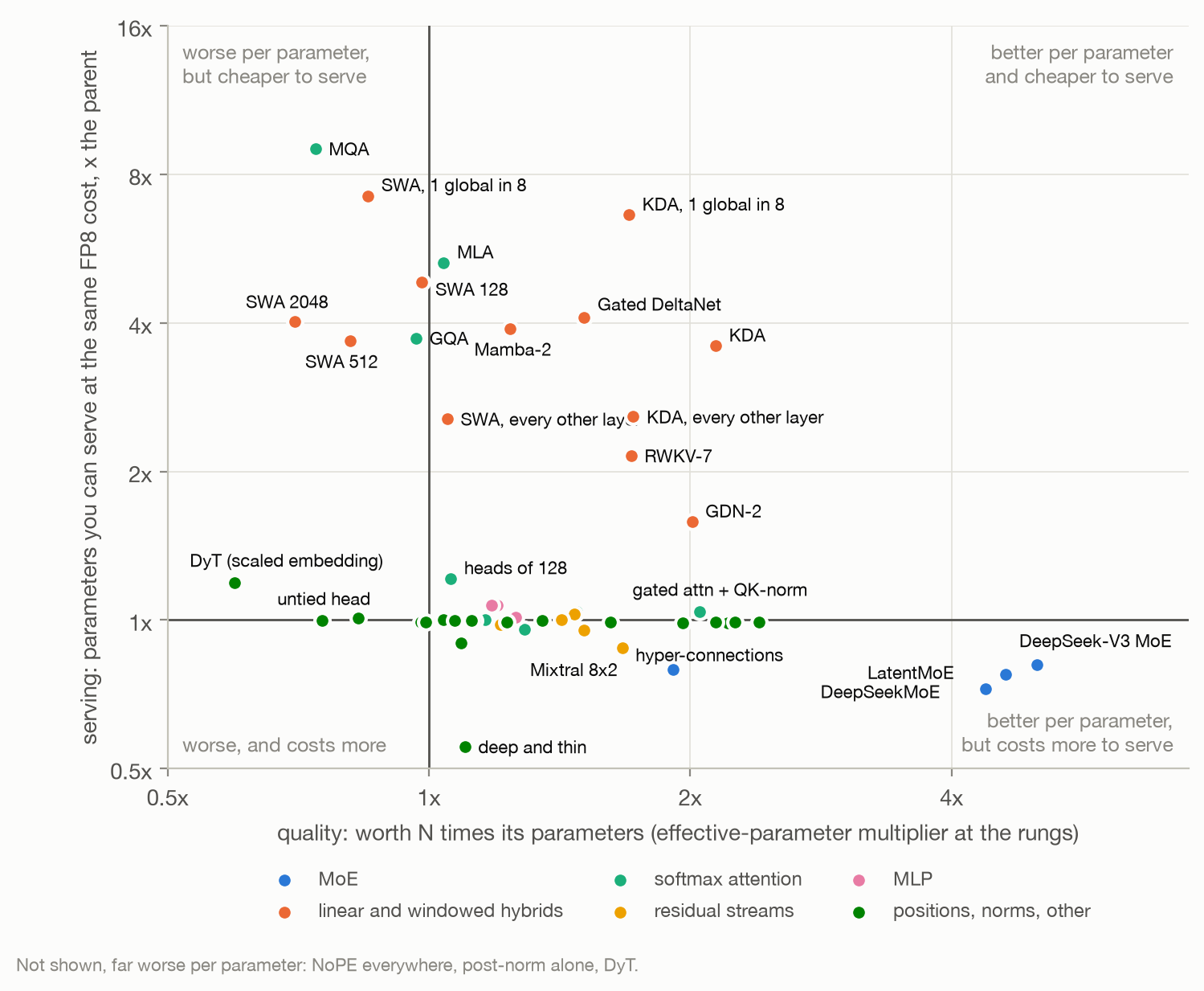
Each dot is one change to GPT-3 + RoPE. Further right means better quality per parameter. Further up means cheaper to serve, which lets me use a bigger model for the same money.
The two things that stand out are fine-grained MoE and linear attention. With MoE, an active parameter does about as much as 4-5 parameters in a dense model. Linear-attention hybrids improve quality per parameter and are also 2-7x cheaper to serve.
Then there's GQA, MQA, MLA and sliding windows. These mostly help by cutting the KV cache. Quality per parameter is a bit worse, but I can serve a 4-9x bigger model. That's a good trade in this setup.
Everything else is much closer together. Norms, MLPs, positions and residual changes do little to the serving cost. Some let a small model match one with 1.2-2x the parameters, but by the size I actually want to serve, that becomes a 1-2% improvement at best. Often it's nothing.
Here's what did best on its own. These are predictions against GPT-3 + RoPE, at equal serving cost and 1T training tokens:
| change | predicted change in loss |
|---|---|
| LatentMoE | -5.7% |
| DeepSeek-V3 MoE (128 experts, sigmoid routing) | -5.5% |
| KDA (one global attention layer in 8*) | -4.8% |
| KDA in 3 of 4 layers | -4.7% |
| DeepSeekMoE (64 experts + shared) | -4.2% |
| Gated DeltaNet in 3 of 4 layers | -4.2% |
| MLA (at DeepSeek's dimensions) | -4.1% |
| 512-token sliding windows (one global attention layer in 8*) | -3.9% |
| Mamba-2 in 3 of 4 layers | -3.6% |
| GQA (4 query heads per KV head) | -3.2% |
* One global layer in 8 at , in 6 at .
#Positional Encodings
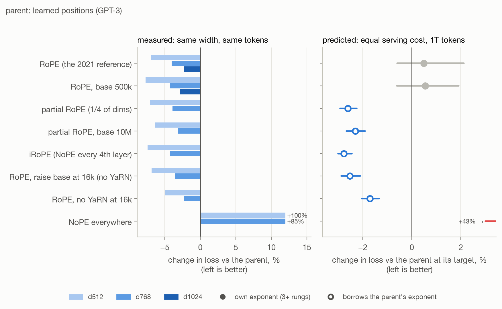
All rows here are against GPT-3's learned table of positions. Positions don't change the serving cost, so there's no serving panel.
RoPE went against my priors here. It starts strong: 6.9% better at . Then the gain shrinks to 4.0% at and 2.3% at . Extrapolate that and it basically disappears: +0.5% at equal serving cost, with a range from -1.0% to +2.1%.
I'd question the setup before concluding that learned positions are fine. Their repository loss also swings from 0.65 to 0.80 across learning rates. I use GPT-3 + RoPE as the reference for the rest of the experiments anyway.
Changing RoPE itself doesn't do much here. A base of 500k, partial RoPE, iRoPE and raising the base at the 16k switch all end up within 1% of plain RoPE at the sizes I trained. My guess is that BPB isn't a good way to tell these apart. I'd want something like RULER.
The hollow -2.5% dots in the plot are misleading. I only trained those variants at two widths, so the fit assumes their advantage over the reference stays the same as the model grows. With plain RoPE I trained four widths, and can actually see the advantage shrinking. I'd expect the variants to do the same. The -2.5% isn't evidence that they beat plain RoPE. Base 500k is a good example of how much the extrapolation matters: it helps at every width I trained, but its advantage shrinks fastest, and the prediction ends up at +0.5%.
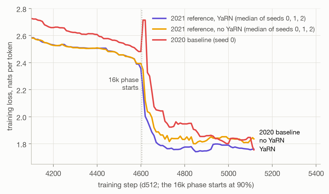
YaRN does matter for using the longer context. Without it, RoPE beats learned positions by 5.3% in the first 2k tokens of a repository, but only 0.6% past 8k.
Removing positions everywhere breaks the model (+100% at ). Removing them from just the global layers of a hybrid is fine, because the local layers still provide position information. The 2026 hybrids do this, and adding partial RoPE back to their global layers is slightly worse (+0.2%). You gotta have some positional inductive bias, but it doesn't need to be in every layer. This part is a quick reproduction of a known result.
#Normalization
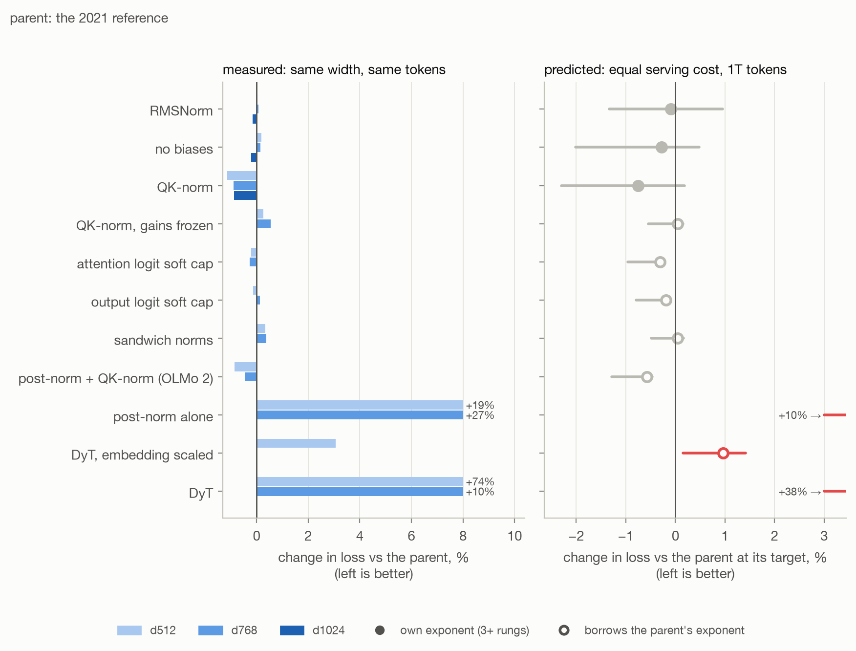
Most of these changes were introduced for speed or stability, and I don't see a quality gain from RMSNorm, removing biases, sandwich norms or logit soft caps.
QK-norm is the exception. It helps by about 1% at every width: -1.1% at , -0.9% at and , and -0.8% at . The prediction at equal serving cost is also -0.8%, though the range crosses zero.
The reference model isn't having loss spikes, so QK-norm gets this gain without fixing an obvious instability. Its attention does get very sharp very early, though: by step 500, the largest attention logit is 71 at lr 2e-3 and 351 at 4e-3. With QK-norm it's 12-25.
Then I removed the learned per-channel scales from the query and key RMSNorms. The gain disappeared: +0.3% and +0.6%, slightly worse than leaving QK-norm out. Letting the model learn how sharp its attention should be seems to be the useful part. Soft-capping the logits to the same range doesn't replace those scales either.
Post-norm alone, x + norm(f(x)), is much worse (+19% and +27%). With QK-norm, as in
OLMo 2, it's fine.
DyT doesn't work with the usual initialization here. With embeddings initialized at 0.02,
tanh(αx) gets tiny inputs. Two of three seeds diverge at (+74%). Multiplying the
embeddings by √d helps, but it's still 3.1% worse.
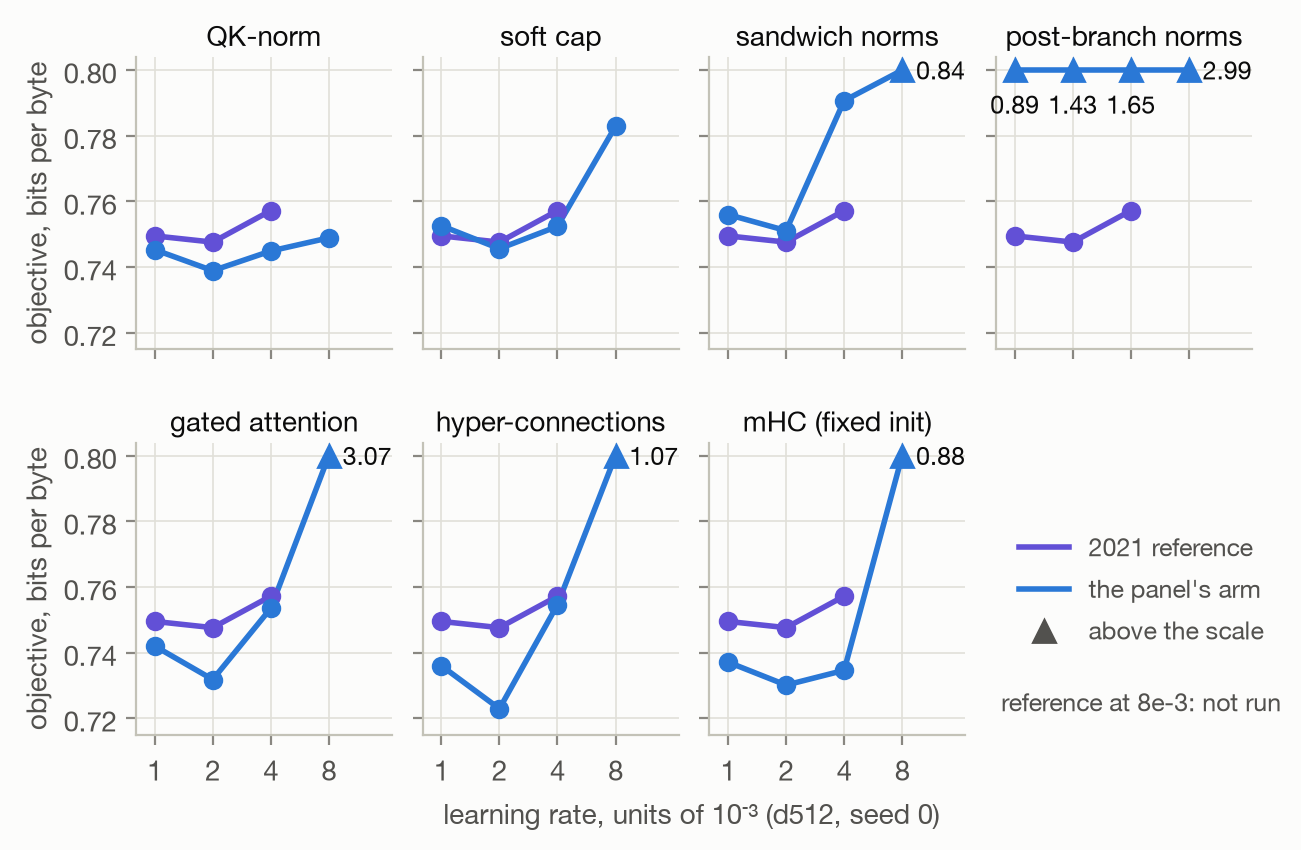
QK-norm also tolerates a higher learning rate well. Going one tested learning rate above its best barely hurts it. Sandwich norms, gated attention and hyper-connections, on the other hand, blow up at 8e-3:
#MLP Variants
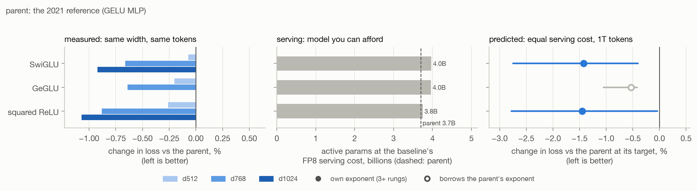
All three alternatives beat the reference's plain GELU MLP (4x wide) at the same parameter count. SwiGLU barely helps at (-0.07%), then improves by 0.66% at and 0.92% at . If I only ran the smallest model, I'd have called it noise.
At equal serving cost, the predictions are -1.5% for squared ReLU, -1.4% for SwiGLU and -0.5% for GeGLU. Serving cost barely changes; the gated MLPs are a bit narrower to keep the parameter count the same.
Squared ReLU wins in the dense model. Put it inside the 2026 hybrid's experts and it makes things 0.7% worse, even with 5% more active parameters. A good dense MLP doesn't automatically make a good expert. I'd still want a second width before ruling it out.
#Softmax Attention Variants
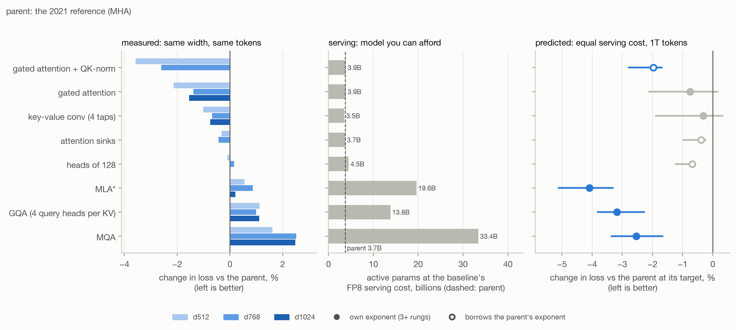
* I trained MLA with a latent of 256 and 32 rotated dimensions. That runs about 2x slower in vLLM than DeepSeek's 512 + 64, which has better kernels, so I used DeepSeek's dimensions for the serving comparison. Keep this in mind if you're considering MLA for a smaller model. You might need to write your own kernels.
GQA makes loss about 1.1% worse at every width, MQA 1.6-2.5% worse, and MLA is within noise. On quality per parameter, there's little reason to switch. Then I measure serving: they cut the KV cache by 4x or more, so the same money buys a 4-9x bigger model. The predictions turn into -4.1% for MLA, -3.2% for GQA and -2.5% for MQA at equal serving cost.
Gated attention, a sigmoid gate on each head's output, improves loss by 2.1%, 1.4% and 1.5% at the three widths. With QK-norm the improvement is 3.6% and 2.6%, slightly more than adding their separate gains. At equal serving cost, the pair is predicted to help by 2.0%.
Inkling's key-value conv, a 4-tap causal convolution over keys and values, helps by 1.0%, 0.7% and 0.7%. I'll get back to it in "Short Convolutions". Sinks and heads of 128 don't make a measurable difference.
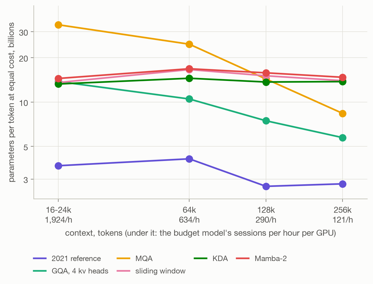
The context length changes which of these I'd pick. At 16-24k, MQA lets me serve the biggest model: 33B. At 256k that falls to 8B, and GQA falls from 14B to 6B. Sliding windows, KDA and Mamba-2 stay around 14-16B:
#Hybrids: SWA vs Linear Attention
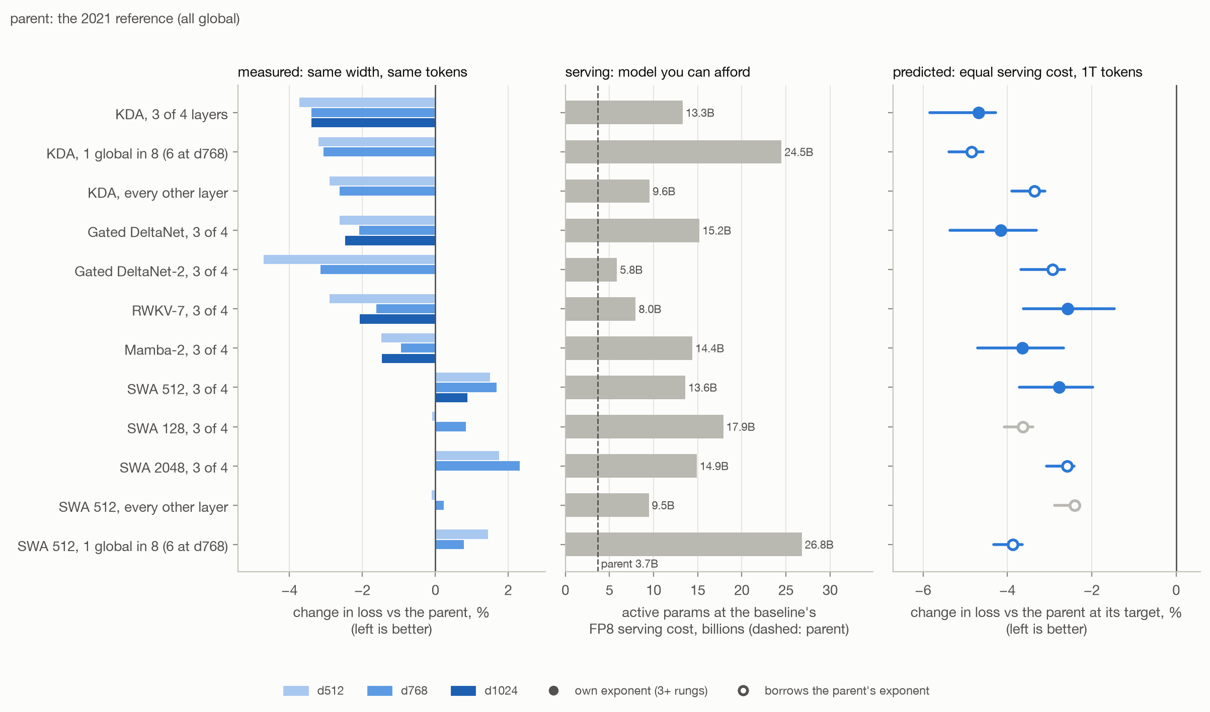
Linear attention is kinda meta here. Replacing 3 of 4 attention layers with KDA improves loss by 3.7%, 3.4% and 3.4% at the trained widths, and lets me serve 3.6x the parameters for the same cost. The predicted improvement is 4.7%. Gated DeltaNet comes next at 4.2%, then Mamba-2 at 3.6% and RWKV-7 at 2.6%.
Sliding windows help through serving cost. Windows of 512 in 3 of 4 layers make quality per parameter 0.9-1.7% worse, but the bigger model I can afford is predicted to be 2.8% better. Windows of 128 are cheaper still and get to 3.6%.
So linear attention looks much better on its own. Then I put MoE, QK-norm and gates into both models, and most of that lead disappears. In the complete late-2026 models, KDA is only a predicted 0.3% better at equal serving cost at 16-24k, and 0.45% at 256k. Most of the improvement comes from the things they share. Maybe that's part of why Western open labs haven't been in a hurry to adopt linear attention.
I also tried changing how many layers use KDA. Three in four and all but one in eight (one in six at ) are within half a percentage point at the trained sizes. The version with more KDA layers is cheaper, but the predictions end up almost the same: -4.8% vs -4.7%. KDA in every other layer does worse. Adding more linear layers lets me serve more active parameters, but the quality tradeoff mostly cancels that out.
A 2048-token sliding window has a different problem. It's only 0.9% worse in the first 2k tokens of a repository, but 9.3% worse past 8k. For the first 90% of training, a window of 2048 on sequences of 2048 is just full attention. Then the 16k phase starts and those layers can suddenly see only 2048 of the 16k keys.
Gated DeltaNet-2 does best per parameter at (-4.7%). Unfortunately, vLLM runs it at 0.42x KDA's speed, bringing the prediction at equal serving cost to -2.9%. I'd be interested in seeing this with better inference kernels. LFM2's short conv is cheaper still, but loses more quality; more on that below.
#MoE Variants
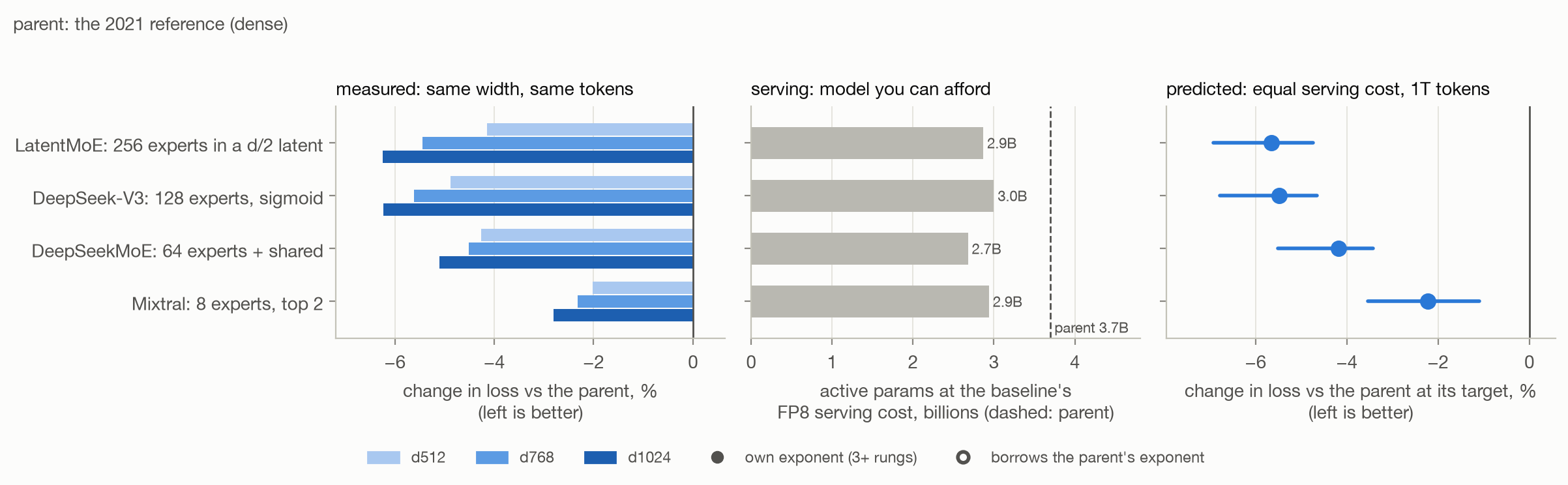
Every MoE here uses the same amount of MLP compute per token as the dense model.
Fine-grained MoE is the easiest win in the whole thing. DeepSeek-V3's 128 experts with sigmoid routing improve loss by 4.9%, 5.6% and 6.2%. Unlike a lot of the small changes, this one gets better with width. A Mixtral-style setup with 8 experts and top 2 gives about half the improvement.
LatentMoE, used in Nemotron 3 and Kimi K3, does a little better still. It projects each token to half the model width, runs it through 12 of 256 experts, then projects it back. The router and shared expert still use the full width. This lets it have twice as many experts as the DeepSeek-V3-like model at the same total parameter count.
At it's behind DeepSeek-V3's MoE (-4.2% vs -4.9%). At they're tied (-6.25% vs -6.23%). At equal serving cost, LatentMoE has the best prediction of any single change: -5.7%.
MoE does cost more to serve per active parameter. With 32 agent sessions running at once, each decoding step reads the weights of many experts. I can afford 3.0B active parameters (33B total) with DeepSeek-V3's MoE, compared to 3.7B dense. It still wins by 5.5%.
The routing details matter much less in these runs. On the 2026 sliding-window model, I tried softmax with a balance loss instead of sigmoid with a bias, removing the shared expert, SMEBU, and sqrt-softplus scores. None made a measurable difference.
On the 2026 hybrid, halving the experts from 256 to 128, still using 7 per token, halves the expert weights read during decoding. The quality difference is small (+0.5% at ). Zero-compute "null" experts are +0.2%, and squared-ReLU experts are +0.7%.
That headline win didn't carry over when I put LatentMoE into the candidate, which already has ordinary fine-grained experts. I used 512 experts, 12 per token, at half the width. The result is within noise: -0.13% at (3 seeds) and -0.11% at (2 seeds). Serving gets a bit slower too: 0.88-0.94x the candidate's sessions per GPU at the same width, leaving room for about 9% fewer active parameters at the baseline's cost.
On the 2021 reference, LatentMoE only caught up with DeepSeek-V3's experts at . Its big win was over a dense MLP; the candidate already has fine-grained experts. I didn't refit with these runs, so there's no prediction at the target. But with no measured gain and a smaller model to serve, it's hard to see one. The final model keeps ordinary experts.
One tuning caveat for the 2021 reference result: LatentMoE's best learning rate there was the lowest I tried (1e-3). But 2e-3 was only 0.02% worse, so it's probably not far off.
#Short Convolutions
Four kinds of short causal convolution show up in this study:
- Inkling's key-value conv: a 4-tap causal conv over an attention layer's keys and values.
- Canon layers (Allen-Zhu, Physics of Language Models 4.1): a 4-tap conv with its own skip, before the mixer (Canon-A) or before the MLP (Canon-C).
- The convs inside linear attention: KDA and Gated DeltaNet run a 4-tap conv over their own queries, keys and values. They're part of each mixer, so I didn't ablate them on their own.
- LFM2's gated short conv: a whole mixer layer built around a 3-tap conv, in place of attention or linear attention.
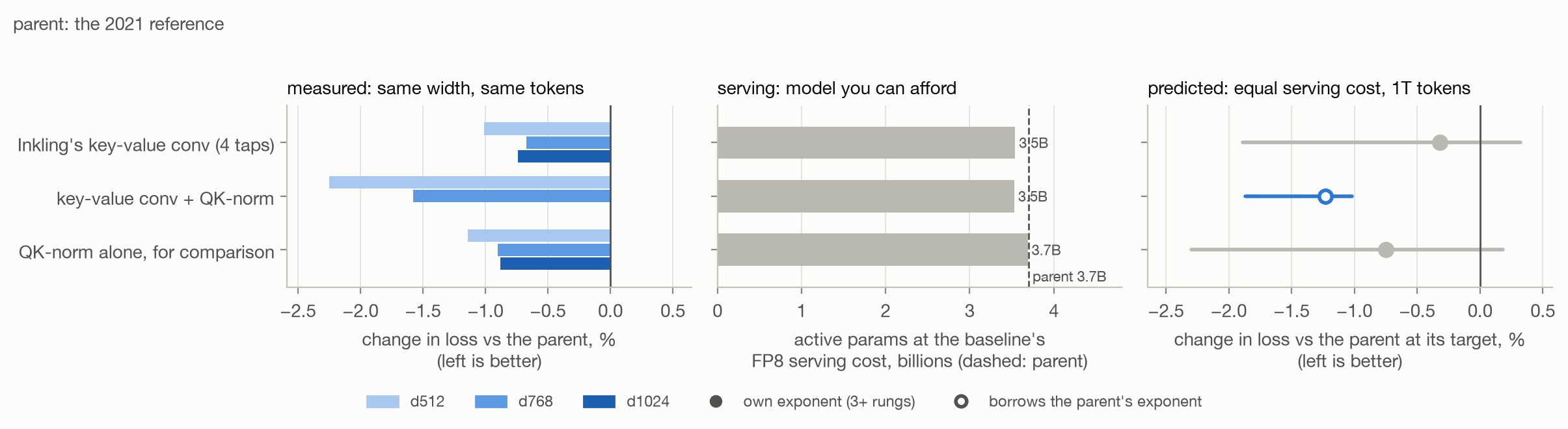
Inkling's key-value conv helps by a small, consistent amount: -1.0%, -0.7% and -0.7% on the 2021 reference. It also reduces the model size I can serve by about 4%, from 3.7B to 3.5B. The prediction at equal serving cost is -0.3%, with a range that crosses zero.
It combines well with QK-norm: together they're -2.3% and -1.6%, about the sum of their separate improvements, and -1.2% at equal serving cost. It also helps on the 2026 hybrid (-0.7% on the global layers). That's K in the first stacking round, and I keep it in the final model.
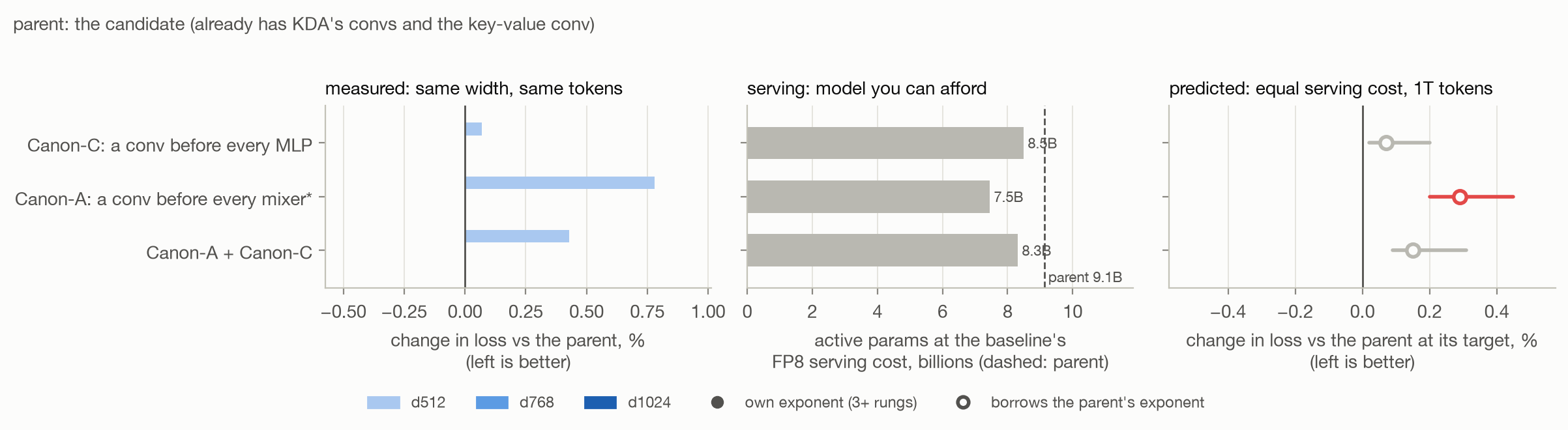
* I didn't benchmark Canon-A's inference speed, so its serving cost is an analytic estimate.
Canon layers don't help the candidate at , the only width I tried. Canon-C is +0.07%, Canon-A is +0.78%, and both together are +0.43%. Replacing HC with AttnRes gives +0.59% for the pair.
But this model already has convs in every layer: inside KDA in 3 of 4 layers, and over keys and values in the rest. Canon's claims about reasoning depth and NoPE matching RoPE are about models without those convs. I didn't test that, so I wouldn't read this as a general verdict on Canon.
LFM2 uses a short conv as the whole mixer. In bux this is short_conv: project the input
to B, C and u, then compute C · conv(B · u), with 3 taps. I tried it in two places.
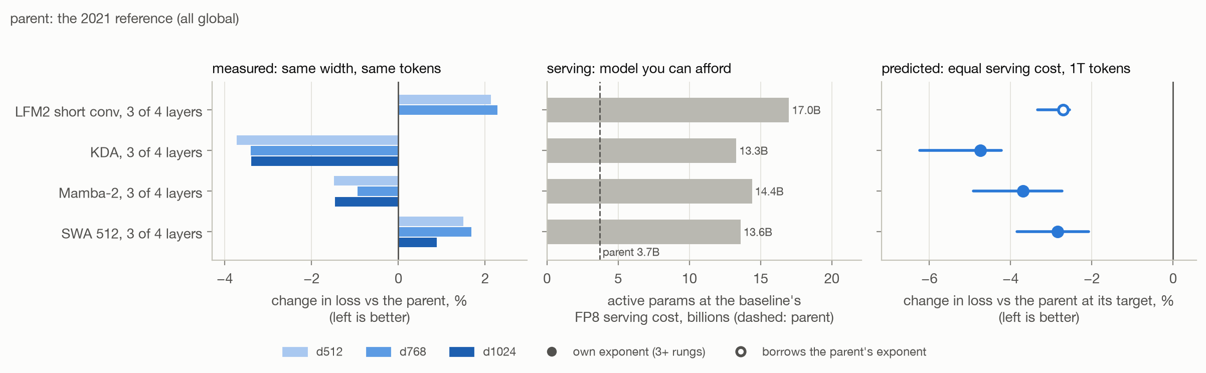
First, I replaced 3 of 4 attention layers in the 2021 reference, the same way I tested KDA and Mamba-2. Loss is 2.1% and 2.3% worse, but serving is very cheap: I can afford 17B parameters, compared to KDA's 13.3B. The prediction is -2.7%, about the same as sliding windows (-2.8%) and well behind KDA (-4.7%).
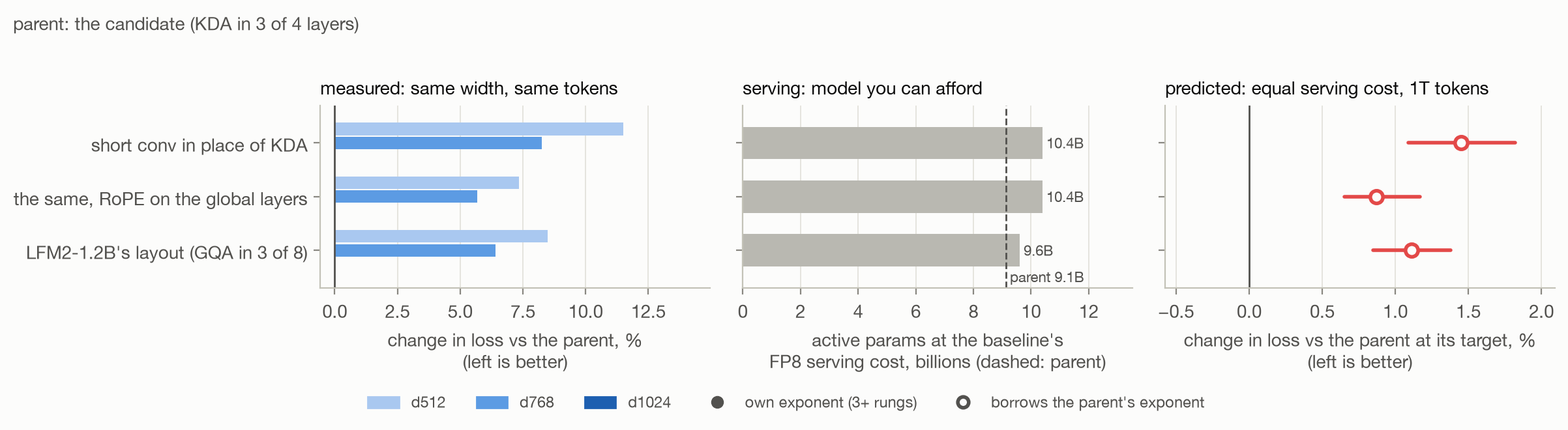
Then I replaced the candidate's KDA layers. This is much worse: +11.5% at , +8.3% at , and +14% past 8k tokens. It does serve about 1.8x as many sessions per GPU at the same width. There are 20% fewer active parameters, and the state is only 0.9 MB per sequence, compared to KDA's 82 MB. But at equal serving cost that only gets me from 9.1B to 10.4B, which doesn't make up for the quality loss. The prediction is +1.45%, with about the same result at every serving context up to 256k.
I also tried LFM2's own layout, with GQA in 3 of 8 layers as in LFM2-1.2B. That's +8.5% and +6.5%. Adding RoPE to the global layers helps a bit (+7.3% and +5.8%), but doesn't change the conclusion. At these sizes, the short conv can't replace what KDA keeps in its state.
#Residual Streams
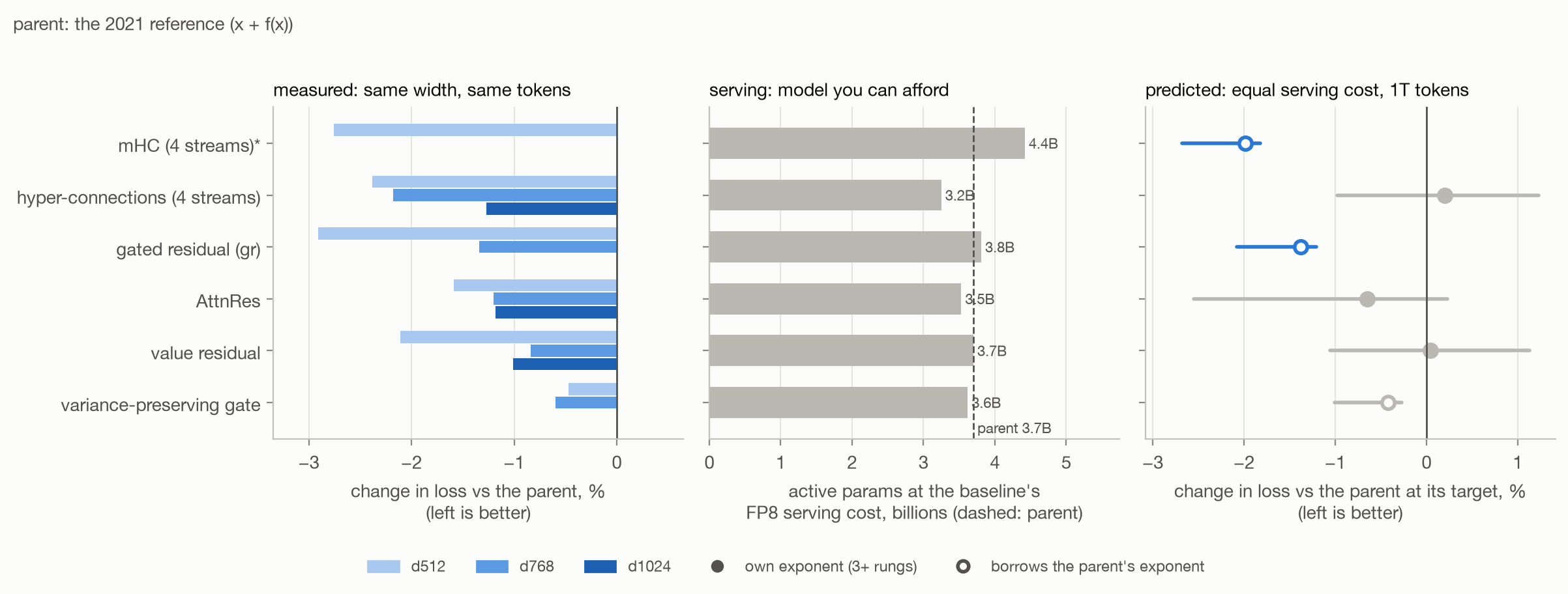
* mHC was run at only on the reference, and its serving cost there comes from the analytic model. On the 2026 hybrid, where it was measured, mHC allows for 19% fewer parameters than hyper-connections.
Hyper-connections keep four copies of the residual stream and learn how to mix them. On the 2021 reference, that improves loss by 2.4%, 2.2% and 1.3%. But even with fused kernels, the extra streams reduce FP8 sessions per GPU by 10%. On the 2026 hybrid it's 20%. For the reference, the serving cost cancels out the quality gain: the prediction is +0.2%.
AttnRes, where each block uses a softmax to mix earlier blocks' outputs, helps by 1.6%, 1.2% and 1.2%. At equal serving cost, the prediction is -0.7%.
The value residual mixes the first layer's values into later layers. It helps by 2.1% at , then 0.8% and 1.0% at the wider models. The prediction at serving size is zero.
Had I stopped at GPT-3 + RoPE, I'd have ruled hyper-connections out. On the 2026 hybrid, they turn out to be the biggest addition in round 1, helping enough to pay for the extra serving cost.
Two residual changes broke at first because of bugs. An initialization bug collapsed mHC's four streams into one. The gated residual (gr) trained to a loss of 2.33 while similar runs were around 0.73; an XLA rewrite on GPUs was halving its residual branch. The results here are after both fixes.
#Sparse Attention
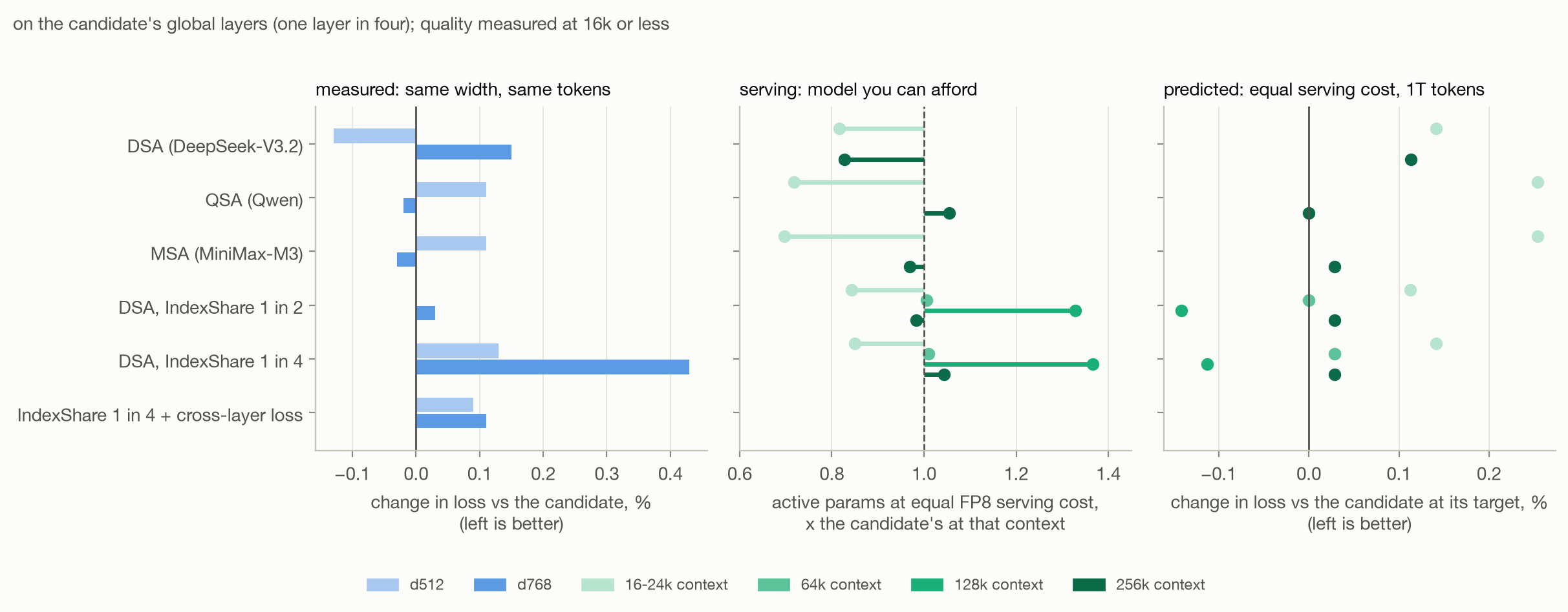
Here I put sparse attention on the candidate's global layers, one in four. Training and quality measurements still stop at 16k. The 64k-256k columns only show how fast the same model serves at longer contexts.
DSA, QSA and MSA don't measurably hurt quality, either here or on the 2021 reference with every layer made sparse. CSA, DeepSeek-V4's compressed sparse attention, is the exception: +8.3% on the reference.
The problem is that at 16-24k, dense FP8 attention is already cheap, and only one layer in four uses it. Running the indexer costs more than the sparse attention saves. At the same serving cost, I can fit only 0.82x the candidate's size with DSA, 0.72x with QSA and 0.70x with MSA.
At longer contexts it starts to help. At 256k, QSA lets me serve a model 1.05x as big. IndexShare runs the indexer in one global layer out of every 2 or 4, then reuses its token choices in the others. That gets to 1.33-1.37x at 128k, though those serving measurements are the noisiest, at ±10%. The quality predictions at equal serving cost all end up within 0.3% of the candidate.
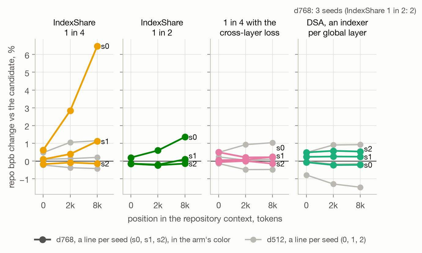
Sharing an index across four layers also failed on one of three seeds. At , that seed was 6.5% worse past 8k tokens because the single indexer drifted during training. IndexCache's cross-layer distillation loss fixed it, giving no measurable quality change on all three seeds.
At 175k tokens, DSA's prefill indexer alone took 3.2 seconds. Running dense FP8 attention took 2.3 seconds. Choosing which tokens to attend to cost more than the dense attention.
#Other (couldn't group)
A few things that didn't fit the sections above:
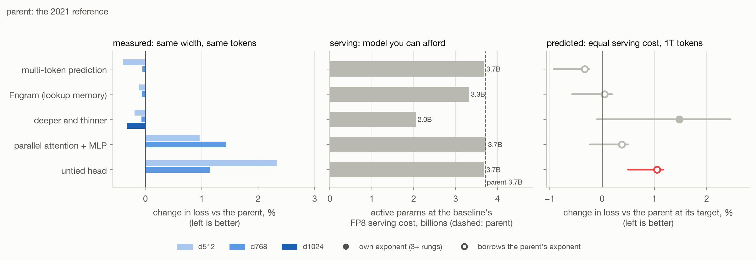
- Multi-token prediction doesn't measurably improve BPB. We saw the same thing in our Mellum2 pre-training ablations: the improvement only showed up on actual benchmarks. MTP is also used for speculative decoding, which I don't measure here.
- Engram, DeepSeek's lookup memory, doesn't help at these sizes.
- Untying the output head makes loss 2.3% and 1.1% worse.
- Running attention and the MLP in parallel makes it 1.0% and 1.4% worse. It might still be worth it if training speed is the priority.
- Making the model deeper and thinner gives the same quality per parameter. But more layers are slower to serve, so the prediction at equal serving cost is 1.5% worse.
#Stacking (round 1)
Next, I want to know whether a change still helps once the model already has everything else.
I start with the 2026 KDA hybrid, a small version of the architecture used by Kimi K3, GLM-5.3-Flash, Qwen3.8 and Nemotron 3. It has three KDA layers per global attention layer. The global layers have no positional encoding, and use QK-norm, an output gate and 4 query heads per KV head. The first FFN is dense; the rest use 7-of-256 experts and a shared expert. There's also one MTP module. This already combines many of the changes above: it's 15.6% better than GPT-3 at , and predicted to be 8.5% better at equal serving cost.
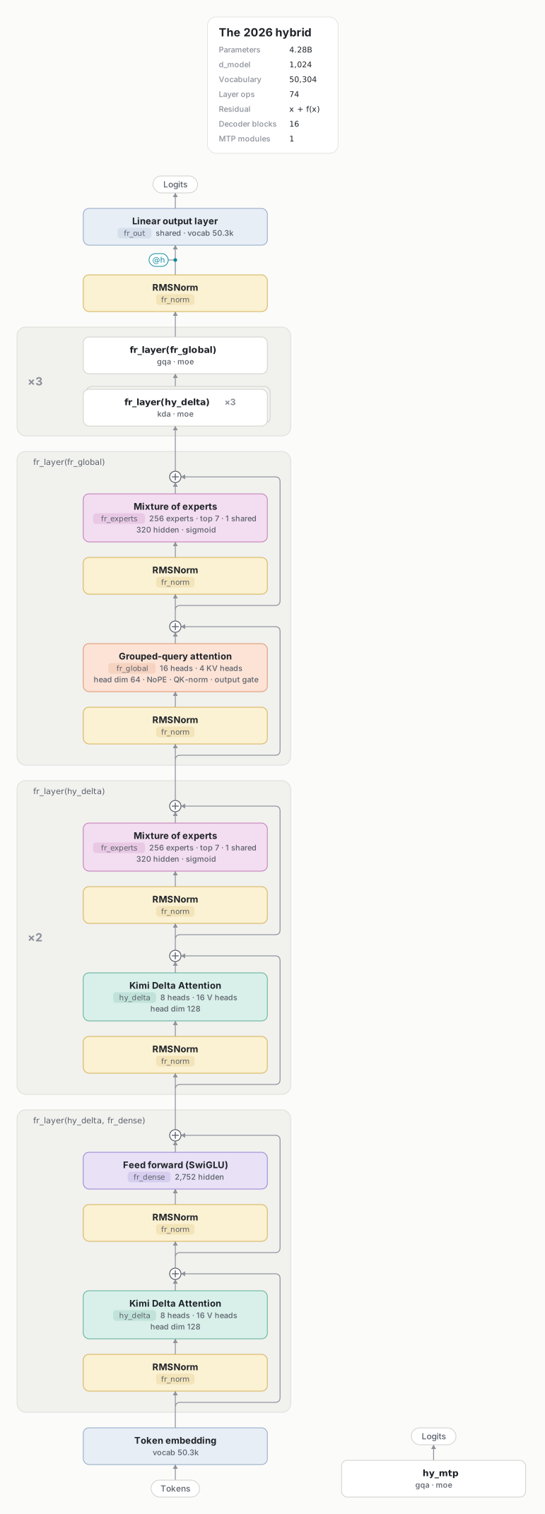
The hybrid: the first FFN is dense, and the remaining FFNs use fine-grained MoE. Diagram source.
For the first round, I picked six things it doesn't have:
- the residual stream: plain, hyper-connections (hc), or AttnRes;
- V: a value residual on the global layers;
- K: a key-value conv on the global layers;
- F: squared-ReLU experts;
- P: partial RoPE on the global layers;
- S: a DSA indexer.
Trying every combination would mean 96 models: three residual options and five changes that can each be on or off. I trained 16 combinations at , with 3 seeds each, balancing the other choices so I could compare models with and without each change. That's a fractional factorial design: enough to estimate each change's average effect without training all 96 combinations.
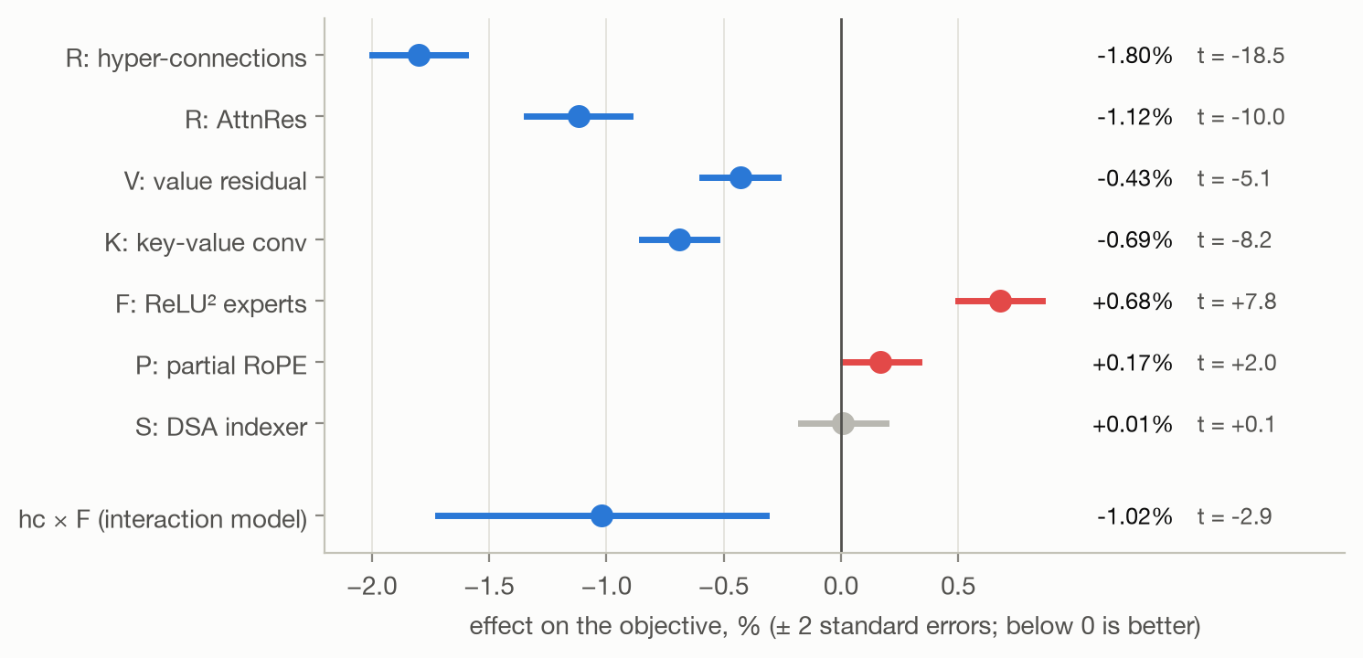
Four options help: HC by 1.8%, AttnRes by 1.1%, K by 0.7% and V by 0.4%. Their gains seem to add up; I don't see interactions larger than the noise. F, P and S are worse or make no measurable difference. The statistical fit suggested keeping F too, but three confirmation runs gave -0.03%, so I left it out.
I went with HC + V + K, which is the model I've been calling "the candidate". Against the hybrid, it improves loss by 2.6%, 2.2%, 1.9% and 1.8% at , , and . The improvement barely shrinks at the last width.
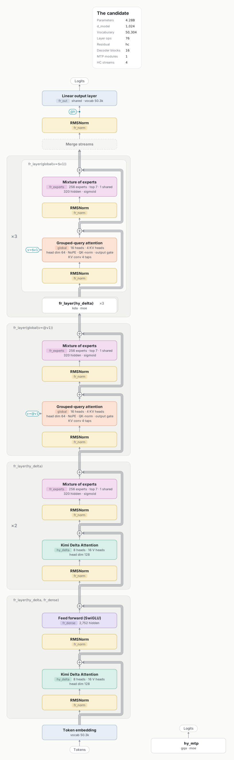
The candidate: HC widens the residual stream to four lanes; v=@v1 saves the first
global layer's values, and v=$v1 mixes them into the later global layers. Each
global layer also has the 4-tap KV conv. The MTP module keeps the hybrid's attention.
Diagram source.
Hyper-connections make it more expensive to serve, so I can afford 9.1B active parameters instead of the hybrid's 11.4B. After accounting for that, the predicted improvement is 0.44%. But it depends quite a bit on the fit. If I give its four widths their own scaling exponent, instead of sharing one with the roughly 60 variants built on it, the improvement becomes 0.96%.
The same problem shows up when comparing HC + V with HC + V + K. Without the conv, the prediction is -0.8%; with it, -0.4%. Serving size barely changes, 9.2B vs 9.1B, and the conv helps by 0.3-0.7% at every width I trained. So I wouldn't use the predicted order to decide whether to keep it. The difference comes from how the scaling laws are fitted together, and I'd call it a tie.
Replacing HC with mHC gives the same quality and better stability at high learning rates, but costs more to serve: 7.4B active parameters instead of 9.1B.
#Stacking (round 2)
For round 2, I tried another four changes on the candidate, labeled stack3 in the plots:
- E: the embedding times √d, as in Gemma and T5;
- G: GatedNorm, a low-rank gate after every norm (Qwen);
- O: a norm on the attention heads' outputs;
- L: a learned value-residual mix.
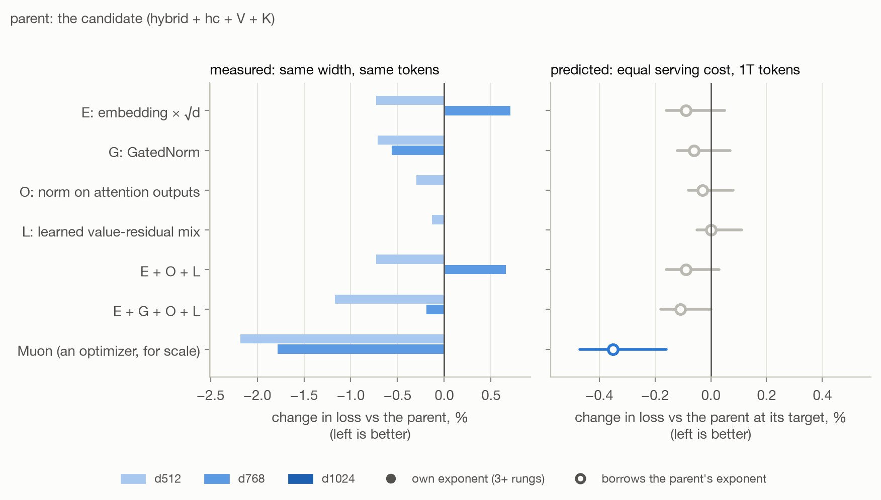
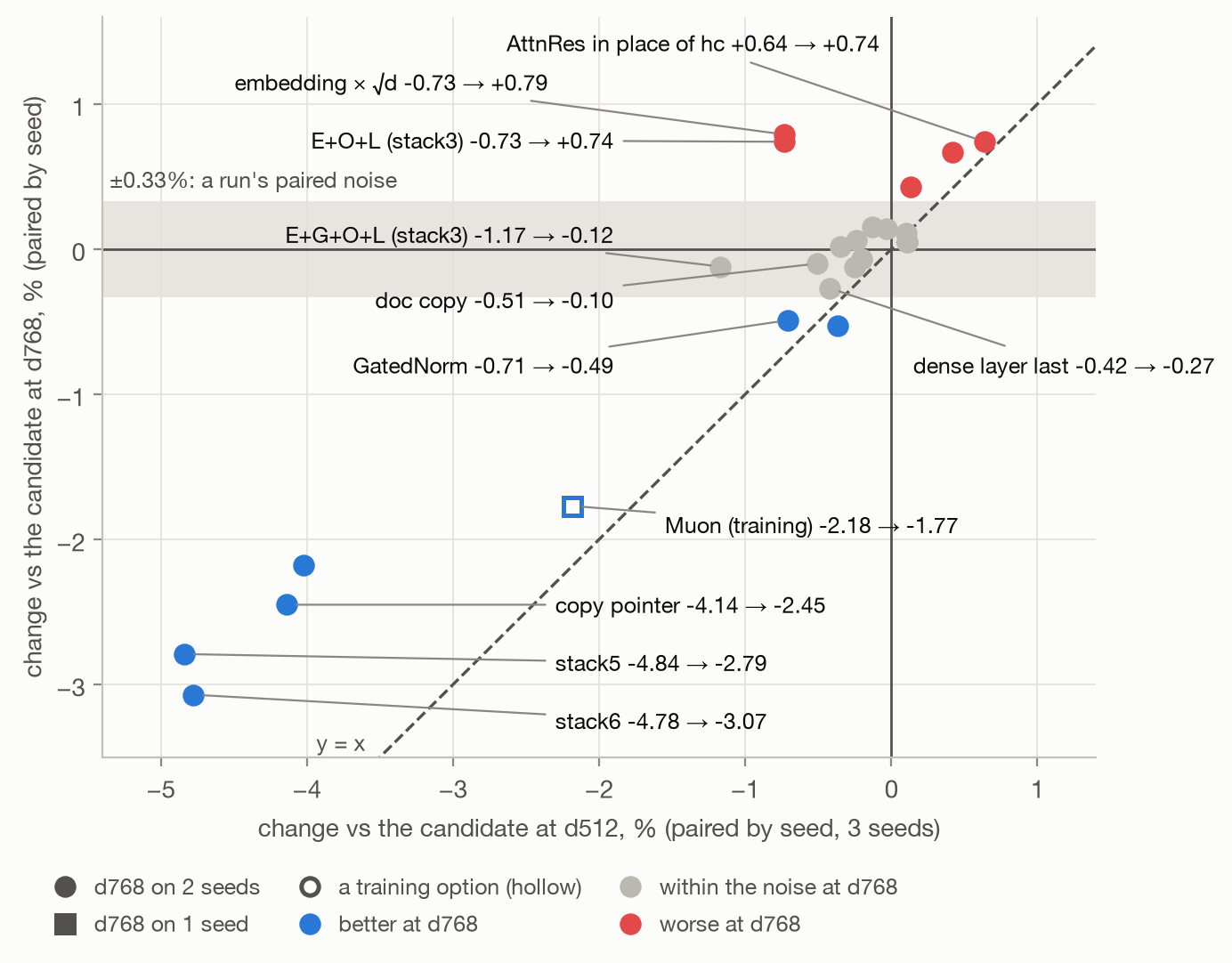
At , all four together look good: -1.2%. At , it's -0.1%, basically gone.
Scaling the embeddings even flips from helping by 0.73% to hurting by 0.79%. Only GatedNorm keeps a gain, going from -0.71% to -0.49%.
For comparison, I also tried Muon, though I kept optimizer changes out of every stack. Its improvement goes from 2.2% to 1.8%. That holds up much better than most of these small architecture changes.
After this, I'd want a second width before adding any change that helps by less than about 1% at .
#Stacking (round 3)
For round 3, I tried more of the new layers from 2026 on the candidate, then combined the ones that helped. I kept the run names in the plots:
- stack4: GatedNorm + value embeddings + learned XSA + differential attention;
- stack5: copy pointer + GatedNorm;
- stack6: copy pointer + GatedNorm + value embeddings + learned XSA + differential attention.
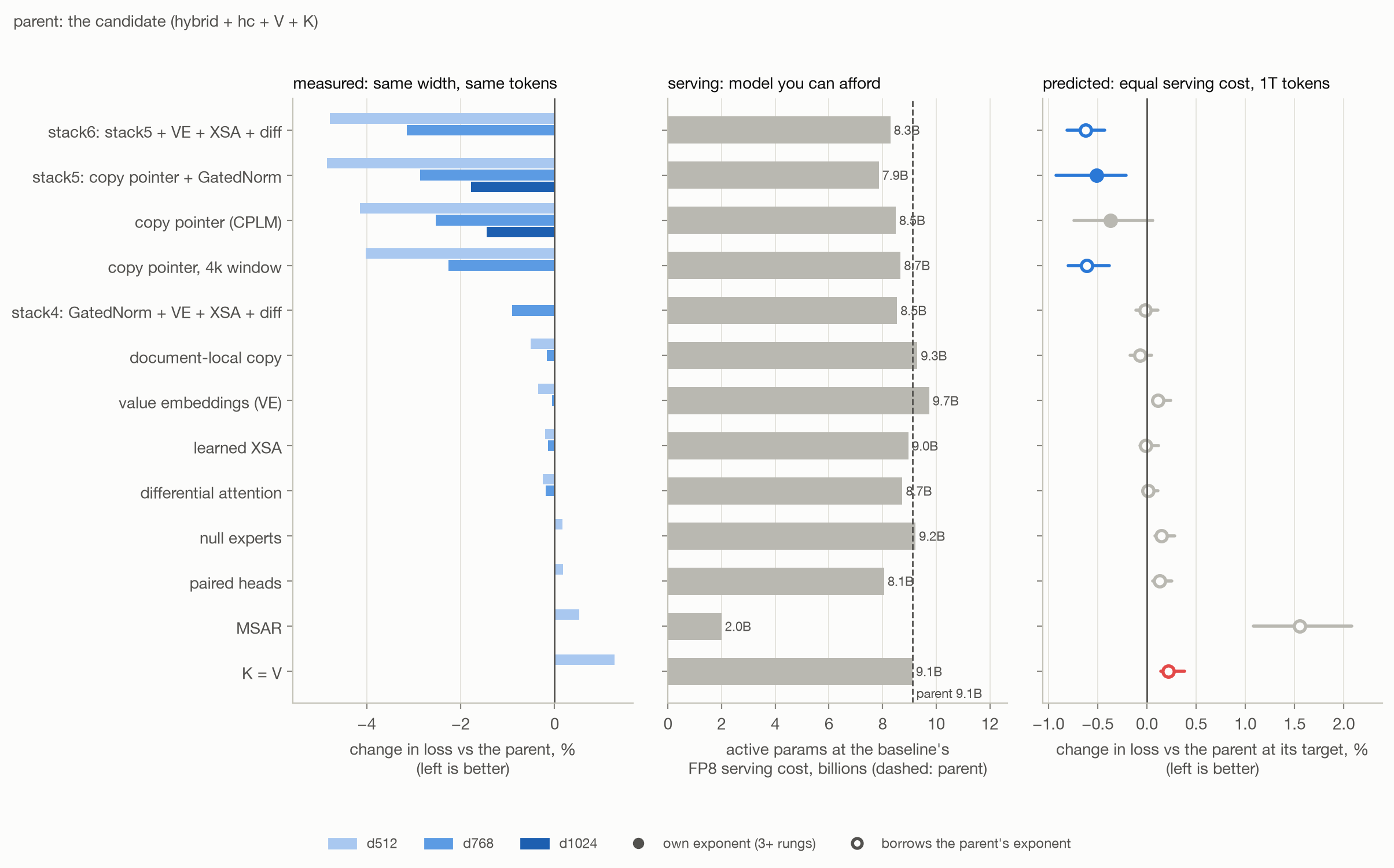
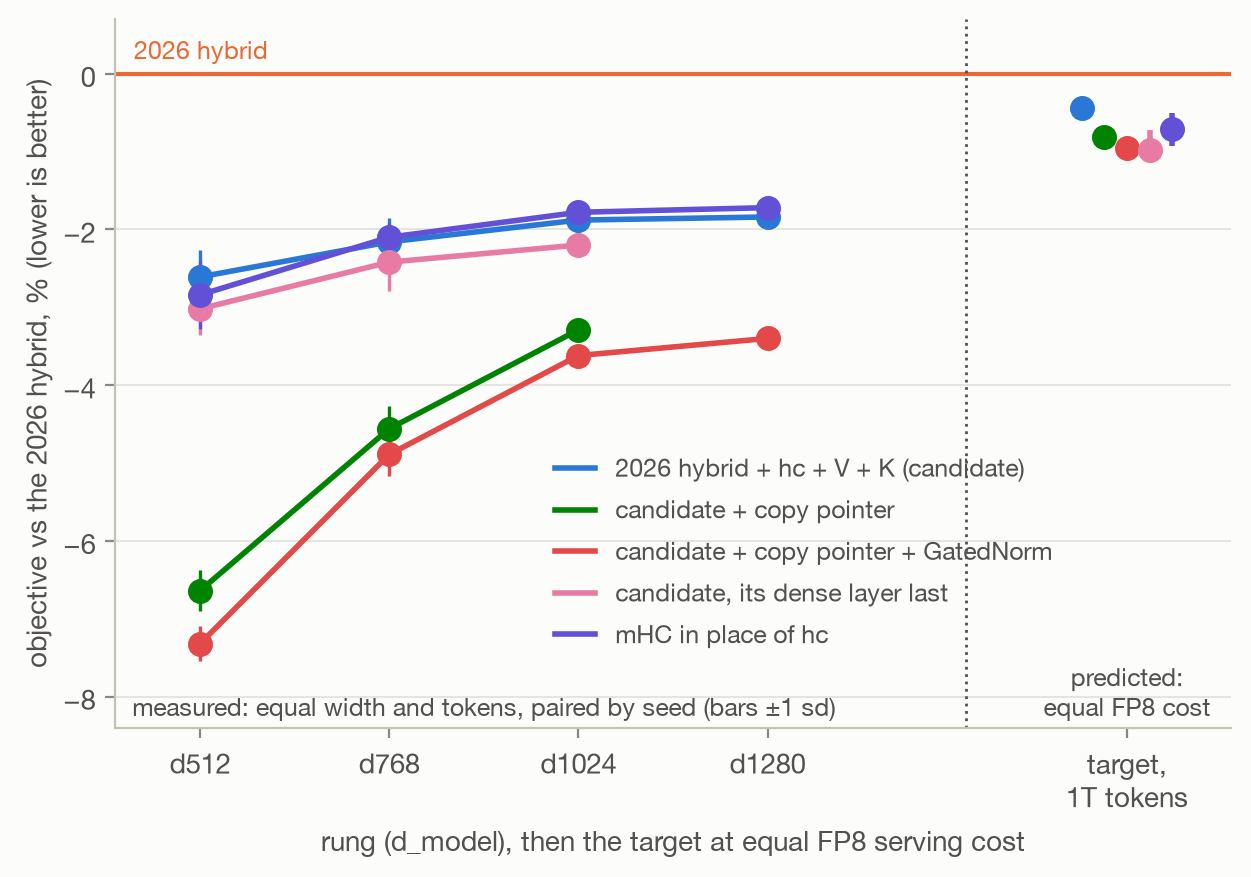
The copy pointer, CPLM from modded-nanogpt, gives the biggest improvement among these additions at small scale. It adds a "copy" option to the output head, letting the model put some probability on copying tokens from earlier in the document. It improves loss by 4.1% at , then 2.5% at and 1.4% at . Each increase in width leaves about 60% of the previous improvement.
With GatedNorm, this becomes stack5: -4.8%, -2.8%, -1.8% and -1.6% across the four widths. The two gains add up fully at and about 95% at . By , the improvement is shrinking more slowly: it keeps 89% of the gain at , compared to roughly 60% between earlier widths. Serving is more expensive, though. I can afford 7.9B active parameters instead of the candidate's 9.1B.
Document-local copy, value embeddings, learned XSA and differential attention lose their gains by . Several other changes are worse:
- K = V is +1.2%, and vLLM still caches both K and V, so it doesn't save serving cost either;
- MSAR is +0.5% and serves 58% fewer sessions per GPU;
- null experts, paired heads and Canon layers also make things worse. Canon is covered in "Short Convolutions" above.
At equal serving cost, the copy pointer is predicted to improve on the candidate by 0.4%, and stack5 by 0.5%. That's too close to the other options to pick a winner from the fit.
The candidate also clips 9-11% of its steps at a gradient norm of 1.0, compared to 0.08% for the hybrid. I blamed hyper-connections at first. Then I looked at where the largest gradient was coming from: the first layer's dense FFN.
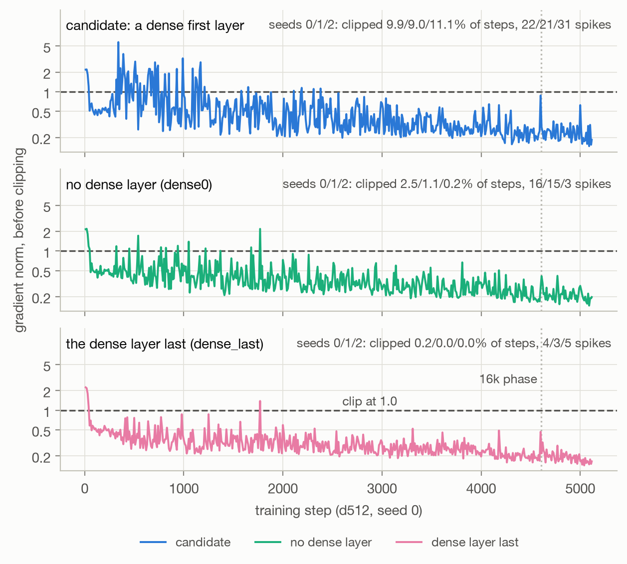
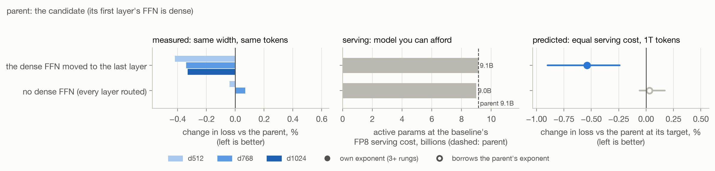
Replacing that dense layer with routed experts, like the other layers (dense0), removes most of the spikes without changing quality. Moving the dense layer to the end (dense_last) removes the spikes too, and improves loss by 0.42%, 0.41% and 0.33% at , and . All 8 seeds improve, and serving cost stays the same.
If GatedNorm is already in the model, the spikes are gone and moving the dense layer doesn't help further.
#The final architecture
After all that, I end up with the 2026 KDA hybrid, plus hyper-connections, a value residual and a key-value conv on the global layers, with the dense FFN moved to the last layer. The prediction is 1.0% better than the hybrid and 9.4% better than GPT-3, at the same FP8 serving cost after 1T training tokens.
Stack5, the candidate with a copy pointer and GatedNorm, is effectively tied with this. Including its run, stack5 predicts -0.95% against the hybrid; the final model predicts -0.98%. I prefer moving the dense layer because it adds no layers, costs the same to serve, and fixes the gradient spikes. The copy pointer benefits from repeated text, which code repositories have plenty of, and reduces the model size I can serve by 14%. Doing both, stack5 with the dense layer last, adds nothing: -0.06% at and -0.05% at .
The bootstrap ranges don't separate them either. Against the candidate, they are -0.54% (-0.90 to -0.24) for the final model and -0.51% (-0.92 to -0.21) for stack5. They overlap almost completely. The final model has no runs in the fit, so I can't tell whether its gain holds at that width the way stack5's did.
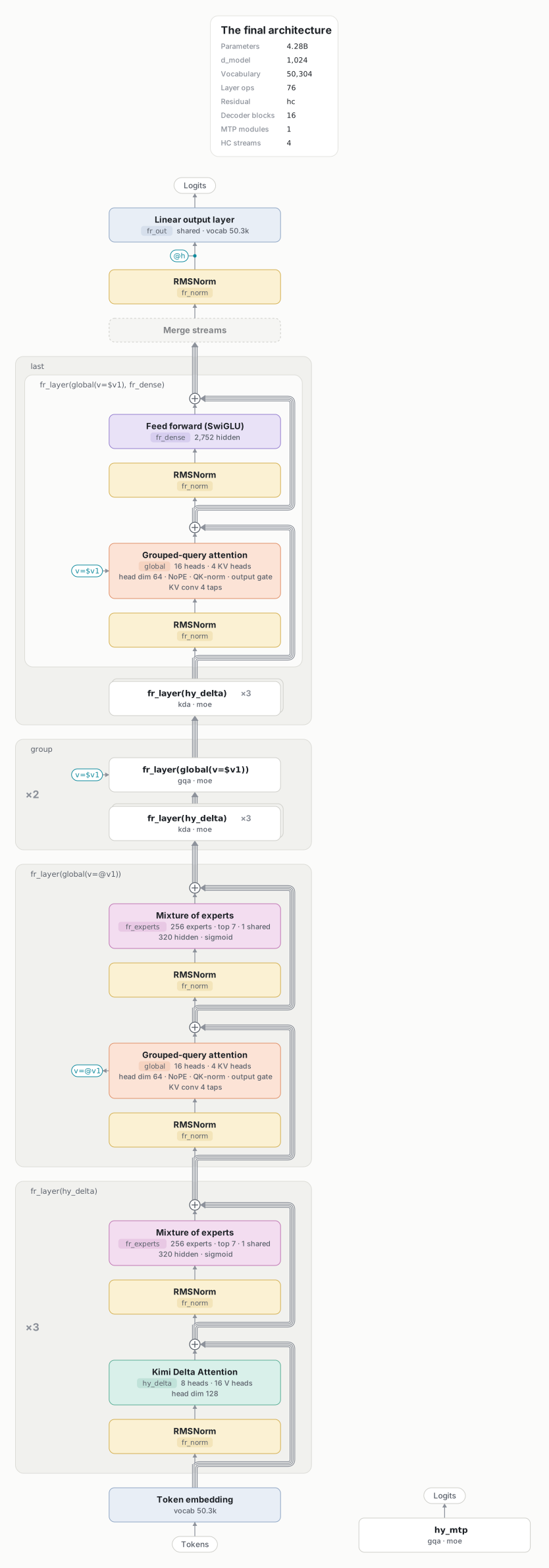
The final architecture: the dense FFN is now in the last decoder block; all earlier FFNs use MoE. HC, the value residual, the KV conv and the MTP module stay the same. Diagram source.
# The final architecture: the late-2026 KDA hybrid with hyper-connections, a value
# residual and a key-value conv on its global layers, and its one dense FFN moved
# from the first layer to the last. Shown at d=1024; any d_model >= 768 works.
d_model    = 1024
vocab_size = 50304
layers     = d_model // 64

norm  = rmsnorm(eps=1e-5)
delta = kda(num_heads=d_model // 128, num_v_heads=d_model // 64, head_dim=128,
            gate_lower_bound=-5)
attn  = gqa(num_heads=d_model // 64, num_kv_heads=d_model // 256, qk_norm=norm,
            gated=true)
glob  = attn(kv_conv_size=4)              # NoPE global layer + 4-tap key-value conv

swiglu_width = (8 * d_model + 96) // 192 * 64
dense   = gated_mlp(intermediate_size=swiglu_width, activation=swish)
experts = moe(num_experts=256, top_k=7, num_shared_experts=1, router=sigmoid,
              routed_scaling_factor=2.5, load_balancing=aux_free,
              aux_loss_coef=1e-4, aux_loss_scope=sequence,
              expert=gated_mlp(intermediate_size=(swiglu_width + 256) // 512 * 64,
                               activation=swish))

layer(mixer, ffn=experts) = [norm mixer] [norm ffn]

# Three KDA layers per global layer. Every global layer after the first mixes the
# first one's values into its own (the value residual: @v1 writes, $v1 reads).
first = layer(delta)^3 layer(glob(v=@v1))
group = layer(delta)^3 layer(glob(v=$v1))
last  = layer(delta)^3 layer(glob(v=$v1), dense)

shared out = head
mtp = $h nextn(norm=norm) layer(attn) norm out   # one MTP module

model    = embed first group^(layers // 4 - 2) last norm @h out mtp
residual = hc(expansion=4)                       # 4 copies of the residual stream

# Training: code and web in rows of 2k, then the last 10% in rows of 16k with YaRN.
tokenizer = tokenizer(name="EleutherAI/gpt-neox-20b")
web       = text(path="data/fineweb-edu/sample/10BT/*.parquet")
code      = text(path="data/stack-edu/files/train/*.parquet")
repos     = text(path="data/stack-edu/repos/train/*.parquet")

data       = 0.6 * code + 0.4 * web
seq_len    = 2048
batch      = 192
budget     = 4.03B                                # tokens: d=1024's rung
steps      = budget // (batch * seq_len)
curriculum = phase(at=0.9, seq_len=16384, batch=batch // 8,
                   data=0.5 * repos + 0.3 * code + 0.2 * web,
                   rope_scaling=yarn(factor=8, original_max_len=2048))

optimizer = adamw(lr=2e-3, weight_decay=0.1)
schedule  = wsd(warmup=0.05, decay=0.2, shape=sqrt)
loss      = loss(z=1e-4)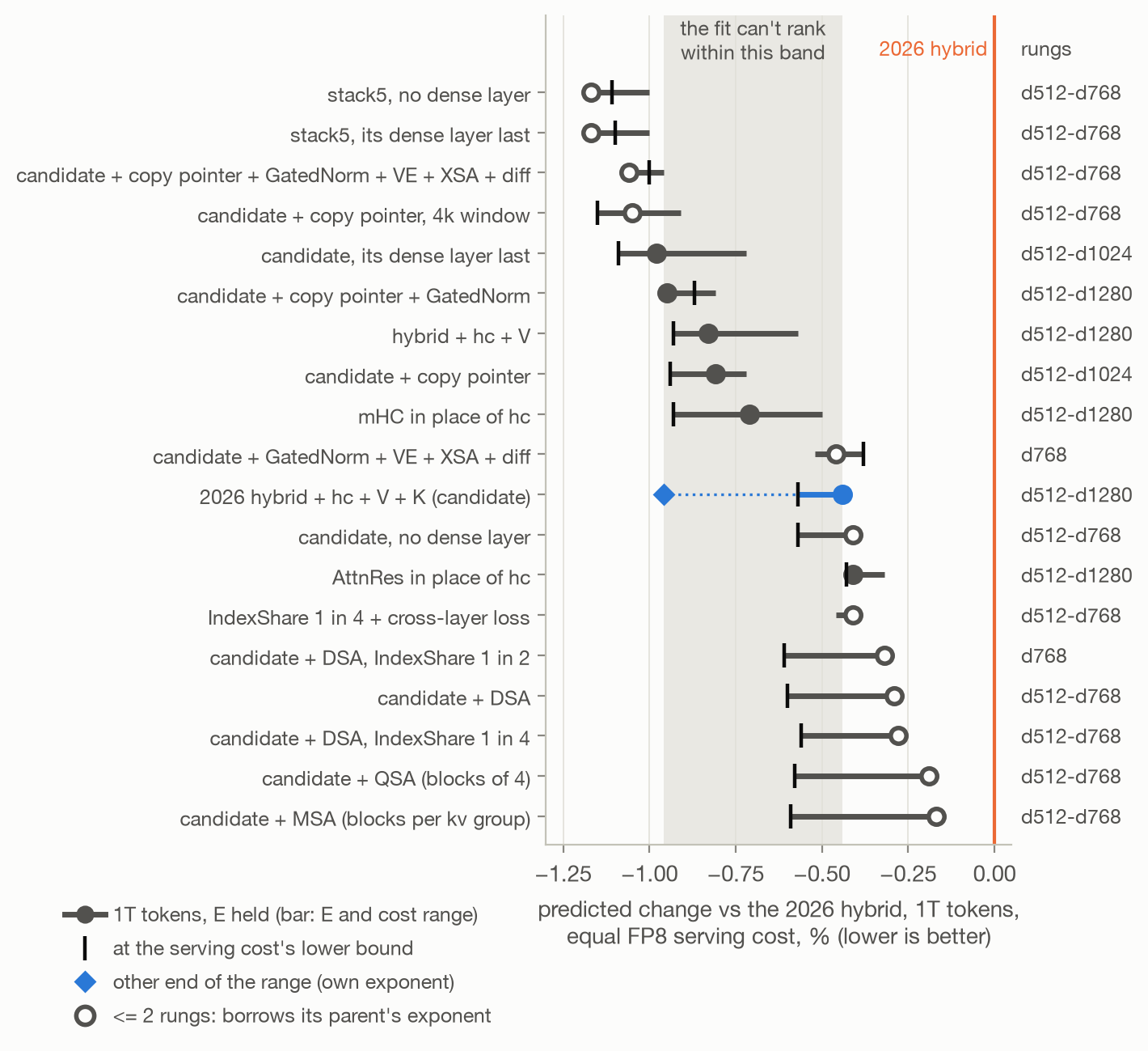
At first glance, the plot says something else: four models sit above the final one, at -1.05% to -1.17%. They are stack5 without a dense layer, stack5 with its dense layer last, stack6, and the copy pointer with a 4k window. All four are hollow dots, though. I only trained them at and . Two sizes aren't enough to see how fast an advantage shrinks, so the fit gives them the candidate's scaling exponent. In effect, it assumes their small-model advantage carries over to big models. It's the same problem as the -2.5% RoPE variants earlier.
The two stack5 variants only move its one dense layer, and at the sizes I trained they're within noise of stack5 itself: -0.14% and -0.02% without the dense layer, -0.06% and -0.05% with it last. But stack5 has four trained sizes, and its advantage over the candidate shrinks from 4.8% at to 1.6% at . The fit sees that and predicts -0.95%. Fit on its two smallest sizes alone, stack5 gets -1.23%, right where its variants are. So among the models with at least three trained sizes, the best are the final model and stack5.
More generally, I wouldn't trust the fit to rank the models near the top. The final model, stack5, the candidate, HC + V, mHC and the copy pointer all end up within about half a percentage point of each other. Their order changes depending on how I fit the models with only a few training sizes. I chose the dense-layer move because it helped at every width tested, with every seed, without a serving penalty.
For the full architectures, the predicted improvements over GPT-3 at equal serving cost and 1T tokens are:
| architecture | change in loss |
|---|---|
| Llama 3 | -4.7% |
| DeepSeek-V3 | -8.4% |
| Qwen3-Next | -8.5% |
| 2026 hybrid | -8.5% |
| final model | -9.4% |
Most of the improvement was already there in DeepSeek-V3, with fine-grained MoE and MLA. The 2025-26 changes look much bigger on the small models I trained than at the size I want to serve.
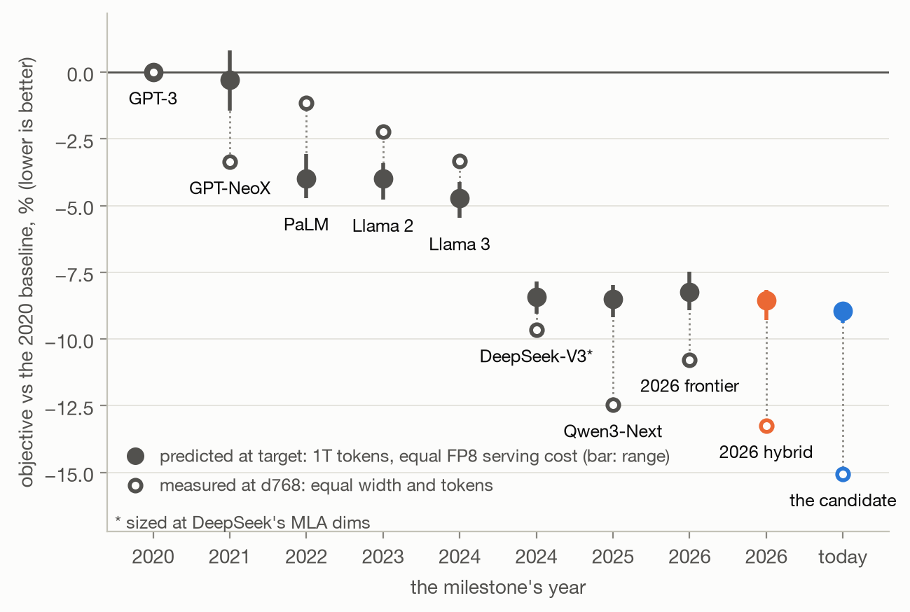
The scaling law leaves the modern model little room to improve through architecture. It splits loss into the entropy of the data, a penalty for limited training data, and a penalty for limited parameters. For the 2026 hybrid at 1T tokens, about 8% of predicted loss comes from limited data and only about 2% from limited parameters. The rest is the entropy of the data itself.
In this fit, architecture can only reduce that last 2%. Even removing the parameter penalty entirely would improve on the hybrid by less than 2%. For the 2021 reference it was about 11%, so there was much more room to improve. That's how a change that makes a model match one with 3x the parameters can end up helping by only half a percent.
Across the experiments, gains at the trained sizes are 1.5-3x larger than the predictions at serving size. The hybrid, for example, beats GPT-3 by 15.6% at , 12.2% at , and a predicted 8.5% at equal serving cost.
Training cost is another way to look at it, if there's enough data available. To reach the hybrid's predicted loss after 1T tokens, the hybrid needs 1.46x as many B300 GPU-hours as the candidate. DeepSeek-V3 reaches GPT-3's loss 2.3x faster than GPT-3 does. Part of that is training efficiency: it runs at 0.26 MFU, compared to 0.16 for the 2026 hybrids.
I also checked what FP8 does to quality on trained checkpoints. Using FP8 weights and KV cache increases code BPB by 0.07% and repository BPB by 0.10%. Pretty small.
The predicted order also holds when I measure serving at contexts up to 256k. Again, quality was only measured at 16k or less:
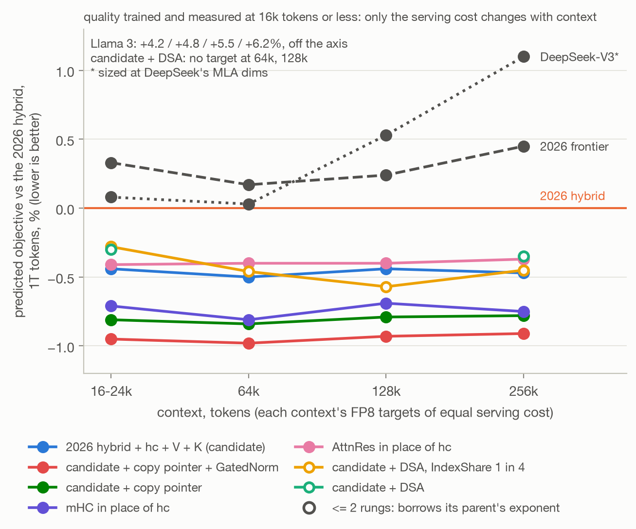
If you serve long contexts, I'd add one more thing: sparse attention on the global layers. The version I'd pick is DSA with GLM-5.2's IndexShare. One global layer in four runs the indexer, and the next three reuse its picks. It's worth training with IndexCache's cross-layer loss. Without it, one seed out of three fell apart past 8k tokens. With it, quality is neutral on all three seeds.
It doesn't pay at 16-24k: at the same width it handles 0.88-0.92x the candidate's sessions per GPU. Only one layer in four is global, and dense FP8 attention is cheap at that length. At longer contexts it does pay: 1.03x at 64k, 1.40x at 128k and 1.10x at 256k. In the predictions at equal serving cost, that's worth only about a tenth of a percentage point, even at 128k. So I see it as a serving option for long contexts rather than an architecture win.
To say anything about quality at 256k, I'd need to train with a 256k extension phase and measure it there.
It's uncanny how close the arch is to Kimi K3. Well, except MLA, but that's largely due to the arch being too small and vLLM not serving the small MLA shapes fast enough. Opus5.5 played a big role in that too, being stupid and giving up on MLA quickly after making this observation.
So I tried MLA again in the candidate's global layers, this time at the shape vLLM serves well on B300: a 576-wide latent on FlashInfer's MLA kernel. It still didn't help. Quality is 1.2-1.4% worse at , on all six seed pairs. Part of that is bux's MLA, which can't take the candidate's value residual, key-value conv or QK-norm. Serving doesn't make up for it either. Even with a 3.1x smaller KV cache in the global layers, it handles 0.78-0.89x the candidate's sessions per GPU at 16-24k, and breaks even at 256k.
I'd give MLA a big chance of making it in too if the target were bigger. However, the diff between GQA and MLA doesn't seem to be mind-blowing.
#Summary
- If you want pure intelligence per parameter out of softmax attention, stick with boring-ass full MHA: it beats GQA, MQA and sliding windows, and MLA only ties it. It's going to be painfully slow to serve though, and that's the only reason those win. The biggest per-parameter wins since 2020 are MoE and linear attention, as long as you only count active parameters.
- Linear attention does seem to work, especially when the kernels aren't an issue anymore. The difference from SWA isn't huge though, so the decision should probably come from smarter signals: actual benchmarks, post-training behavior analysis, etc.
- Residual streams work, though hyper-connections only pay for their serving cost on the 2026 hybrid, not on the 2021 reference.
- Overall, the progress of architecture research does show up even in such small-scale experiments. People's work isn't useless.
To be fair though, the SOTA training setup on a mid arch can completely obliterate the best arch on a mid setup. Take Muon, for example: just swapping the optimizer buys about as much as a whole round of architecture stacking. I'd expect similar gains from data tweaks. So in a sense, arch research seems to be a privilege of labs that have everything else sorted out.
#A Side Note: How Good AI Is at Research
Opus5.5 could implement an architecture from its tech report in under 30 minutes. That would've taken me a day or so. It debugged complex XLA issues and kernels, understands good research practices, and is quite good at googling.
Then it would miss the most obvious combinations, even after seeing that the individual changes were amazing. When asked why, it would say "yeah, I guess worth trying". That can feel like gaslighting: a gigabrain doesn't do something obvious, so you start questioning yourself, maybe you're too stupid to see why it's a bad idea.
I think AI's gonna get better at this pretty soon too, the same way it did at coding.
P.S. I was running Claude Code and Codex inside Air in PyCharm. Gonna give the colleagues credit, it's really nice.
#To reproduce:
- Framework: bux.
- every
.buxfile of the study:examples/experiments/timeline/; - the training recipe:
timeline_code.bux; - the walkthrough:
docs/tutorials/timeline.md; - the scaling-law fit:
scripts/timeline/fit.py.
- every
- Train one family's ladder:
bux launch examples/experiments/timeline/dense_last.bux. Export it for vLLM:bux export examples/experiments/timeline/dense_last.bux OUT. - Open data:
pavlichenko/bux-timelineon Hugging Face, under CC BY 4.0. It has all 1,129 runs, each with a self-contained.bux, its rerun commands and its logged curves, plus 5,232 vLLM serving measurements and both refits with their inputs. Browse the runs online, or download the pack and open itsindex.htmloffline. - Training curves: W&B project.
- Scale: 1,129 training runs from October 27 to 30, about 1.1T training tokens. At most ~112 B300 GPUs ran at once, for roughly 2,800 GPU-hours (an estimate, not counting the serving sweeps).